Microscope parameters

There are a multitude of simulation parameters that can be set. For the purpose of organisation, these parameters have been split onto various panels (and dialogs).

Microscope

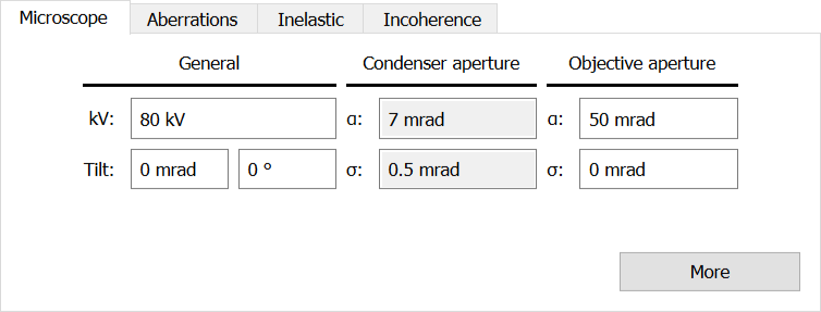
Figure The microscope panel from the main interface.

This section defines the characteristics of the microscope without aberrations, including accelerating voltage, beam tilt and apertures. The beam tilt is defined using a tilt angle in mrad and an azimuth in degrees. The azimuth is measured from the x-axis. The apertures are defined using the semiangle, α, in mrad and a smoothing factor, σ, that describes the radius of a smooth transition from 1 to 0 at the aperture’s edge. Note that condenser apertures are only used in STEM/CBED and objective apertures are only used in CTEM imaging.

Aberrations

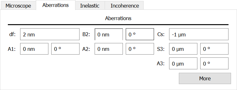
Figure The aberrations panel from the main interface.

The aberrations can be set via the aberrations panel. Complex values are set using magnitude and phase values. Note that there are more aberration coefficients in the Aberrations dialog. It is important to note that the notation used is the Krivanek notation in the dialog, but the Uhlemann and Haider notation in the main interface panel. However, some variables have a factor between the two notations, clTEM does not include this and only works from the Krivanek notation (even if the entry box label uses a different notation)

Aberrations dialog

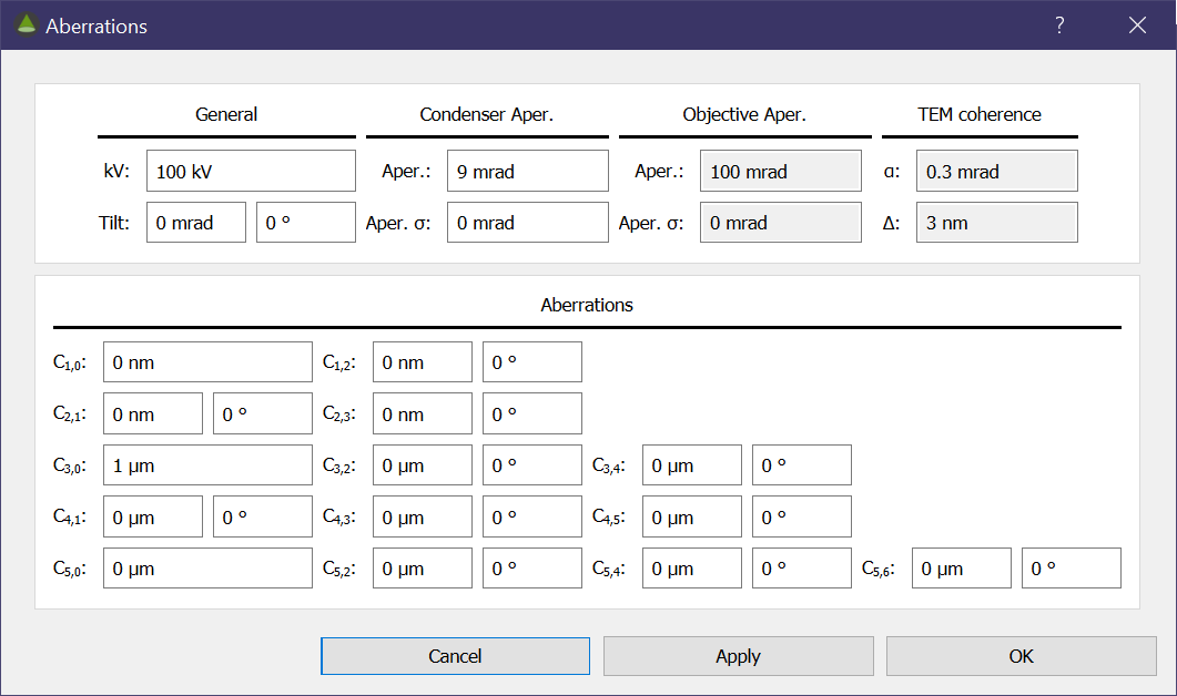
Figure The aberrations dialog.

The aberrations dialog contains the same information as the Microscope and Aberrations panels with more aberration coefficients. It can be accessed from the menu bar or by pressing the ‘More’ buttons on the Microscope or Aberrations panels. There are also TEM coherence settings that are discussed in the coherence sections below.

Inelastic scattering

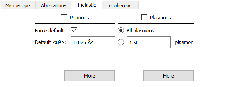
Figure The inelastic scattering panel.

The inelastic scattering effects can be split into two section: The (frozen) phonons and plasmons. These effects require simulation multiple times (the number of which is defined in the Run panel) and averaging the results. Because of this they will drastically increase the time taken for a simulation.

Frozen phonons

Frozen phonons are used to model the effects of thermal diffuse scattering. This is particularly important for STEM and CBED simulations where the intensity within the diffraction plane is drastically modified by the thermal diffuse scattering. The frozen phonon approximation works by slightly adjusting the position of each atom and simulating, which is repeated for every iteration. The magnitude of the displacement is defined by the thermal parameters, <u²>, which defines the variance of the displacement probability normal distribution. These values will be read in from input files if they are defined or you can set the from the interface. From the main interface panel, you can toggle the frozen phonons on and off and you can define a default <u²>. There is a checkb-ox to force this default value over any other defined values. Clicking on ‘More’ shows the phonon dialog where more specific values can be set.

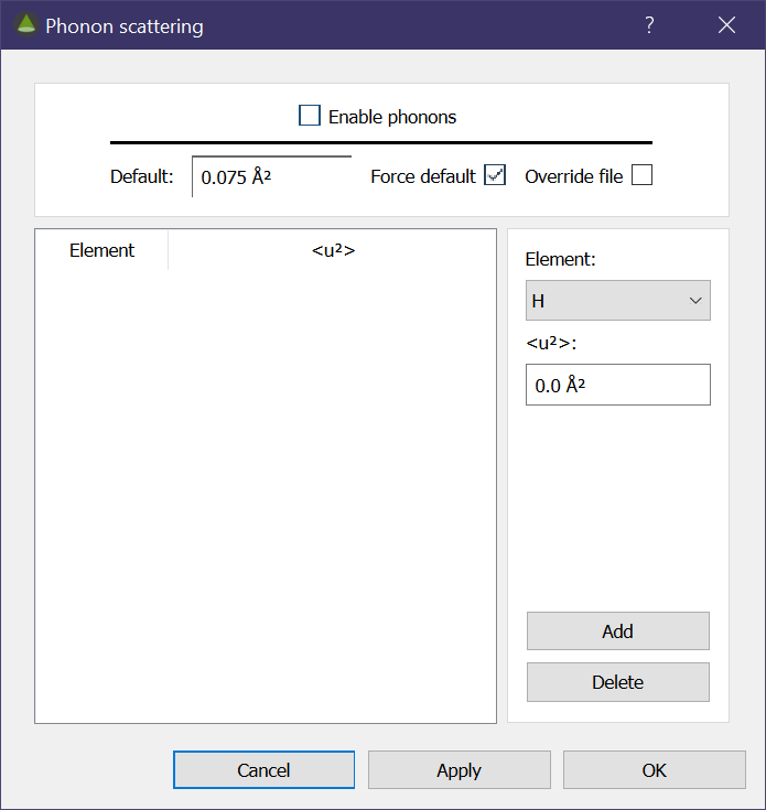
Figure The frozen phonon dialog.

At the top of this dialog is the same enable/disable toggle as well as the default value and check-box to force the default. There is also an override file check-box that will override file defined values with any values defined in this dialog.

The main section of this dialog allows you to define thermal parameters per atom type. This is done by selecting the atom symbol from the drop-down box and typing in the value. You can then click add to set this value and it will appear in the table on the left. Note that the thermal parameters can only be defined per element, not per atom position. The thermal vibration can only be set isotropically.

Plasmons

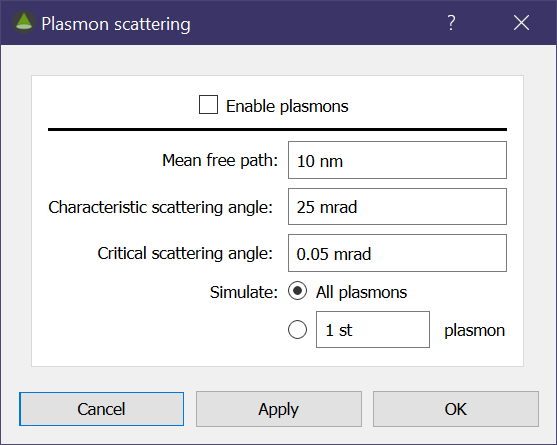
Figure The plasmon dialog.

In the plasmon dialog the plasmon simulation can be enabled/disabled as well as setting the mean free path, characteristic angle and critical angle. For further information see reference 7. There is also the option to simulate all plasmons or a single plasmon. For all plasmons, the scattering depths are determined randomly and these are used no matter how many scattering events they produce. Note that because the scattering depths are determined by the mean free path, the all configuration could not include any plasmon interaction (e.g. for a small sample or a large mean free path). For the single plasmons, it may not be possible to achieve the desired number of scattering events, in which case a warning will be shown when you attempt to run a simulation.

On the main user interface, the option to choose the plasmon number, or all plasmons, is presented. This still requires the parameters within the dialog to be set.

Incoherence effects

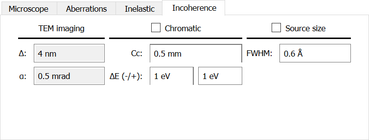
Figure The Incoherence panel.

This panel lets you set incoherence effects. These are divided into three main sections.

TEM imaging incoherence

These parameters are used to calculate the partial spatial and temporal coherence effects and are included in the CTEM image calculation only. Δ defines incoherence effects such as fluctuating beam energy and lens current. α defines the spatial incoherence from the beam convergence (i.e. when it is not perfectly parallel).

Chromatic effects

Chromatic effects are only used in CBED and STEM simulations. First you must define the chromatic aberration coefficient and the energy spread half-width-half maximum (HWHM). The HWHM are separately defined for negative (first entry box) and positive widths (second entry box). These values then calculate a change in focus that is applied. This is repeated for the number of iterations defined in the Run panel and the results are averaged incoherently.

Source size effects

Source size effects are only used in CBED and STEM simulations. The source size full-width-half-maximum is defined and is then used to randomly perturb the probe beam position. The outputs are incoherently averaged. Note that this is not the typical source size is incorporated into STEM simulations, where the output image is convoluted with a Gaussian representing the source size. The method used here is much slower and is therefore largely for use in CBED simulations.